114. Investment Under Uncertainty#
In addition to what’s in Anaconda, this lecture will need the following libraries:
!pip install quantecon
114.1. Overview#
This lecture studies Lucas and Prescott [1971], a paper that helped to ignite a rational expectations revolution.
Lucas and Prescott studied a competitive industry in which
demand shifts randomly each period
firms face costs of adjusting their capital stocks
firms must forecast future prices in order to decide how much to invest
the probability distribution that firms use to forecast prices equals the probability distribution that their investment decisions actually generate
That last bullet point is what Muth [1961] called rational expectations.
The QuantEcon lecture Rational Expectations Equilibrium presents what we might call a “baby” version of the Lucas-Prescott model.
That lecture studies a linear-quadratic industry without uncertainty.
The present lecture describes the more ambitious structure that Lucas and Prescott actually built.
Relative to the baby version, Lucas and Prescott
let demand be shifted by a Markov process \(\{u_t\}\), so that the equilibrium is a stochastic process rather than a deterministic path
allow a nonlinear technology for converting investment into capacity
prove that a competitive equilibrium exists and is unique
show that the equilibrium is the solution of a planning problem that maximizes discounted consumer surplus
show that the equilibrium is a Markov process in the state \((k_t, u_t)\)
provide conditions under which that Markov process has an invariant probability distribution to which it converges from any initial condition
The last item is the part of the paper that most influenced later work.
A model whose equilibrium is a Markov process with an invariant distribution is a model that can be taken to time series data.
That observation set the stage for the rational expectations econometrics subsequently developed by Lars Peter Hansen and Thomas Sargent [Hansen and Sargent, 1980].
Along the way we’ll describe how Prescott and Mehra [1980] later distilled the Lucas-Prescott structure into a general definition of a recursive competitive equilibrium.
The sequel Optimal Growth Under Uncertainty and Tobin’s q studies a paper that asks the same questions about a one-sector optimal growth model, Brock and Mirman [1972], and a paper that uses that model to think about Tobin’s \(q\), Sargent [1980].
Let’s start with some imports:
import numpy as np
import matplotlib.pyplot as plt
import quantecon as qe
from collections import namedtuple
114.2. The industry#
An industry consists of many small firms.
Each firm produces a single output \(q_t\) with a single input, capital \(k_t\).
Production has constant returns to scale, and with a suitable choice of units the production function is
Because capital is the only input and output is sold at a positive price, every firm produces at capacity, so that \(q_t = k_t\).
Let \(x_t\) denote gross investment.
Capacity next period is related to capacity this period and investment by
where \(h\) is bounded, continuously differentiable, increasing, and strictly concave.
The strict concavity of \(h\) is what creates costs of adjustment: doubling the rate of investment per unit of capital less than doubles the resulting increment to capacity.
Adjustment costs are why firms change their capital stocks gradually instead of jumping immediately to a long-run target.
Assume that \(\delta = h^{-1}(1)\) exists and satisfies \(0 < \delta < 1\).
Then \(x_t = \delta k_t\) is the investment rate that just maintains capacity, so \(\delta\) plays the role of a depreciation rate.
Let \(p_t\) be the output price and let \(\beta = 1/(1+r)\), where \(r > 0\) is the cost of capital.
The present value of a firm is
Because the allocation of a given industry capital stock across firms does not matter, we can use \(k_t, x_t, q_t\) interchangeably for firm and industry variables.
Equivalently, we can think of a competitive industry with a single price-taking firm.
Industry demand is subject to random shifts:
where \(D\) is continuous and strictly decreasing in \(q_t\) and increasing in \(u_t\), so that an increase in \(u_t\) shifts the demand curve to the right.
The demand shifter \(\{u_t\}\) is a Markov process with transition distribution \(p(\cdot, u)\), meaning that the probability that \(u_{t+1} \in A\) conditional on \(u_t = u\) is \(\int_A p(dz, u)\).
114.3. The firm and the price of installed capital#
Before studying equilibrium, Lucas and Prescott pause over an instructive question: what does an individual firm actually need to know?
Let \(w_t\) be the current market value of a unit of installed capital and let \(w^*_t\) be the value per unit expected to prevail next period.
A firm that begins period \(t\) with capital \(k_t\) and invests \(x\) obtains next-period capital worth \(\beta k_t h(x/k_t) w^*_t\) at a cost of \(x\), so it solves
The current value of the firm is
and the first-order condition is
Solving (114.5) and (114.6) jointly for \(x\) and \(w^*_t\) gives an investment function of the form
Lucas and Prescott note that (114.7) is essentially the investment function that Grunfeld had used in empirical work, with the market value of the firm as an explanatory variable.
Their argument is stronger than Grunfeld’s, though: a firm does not need to forecast its own future income stream at all.
It needs only to know the value that securities markets place on a unit of installed capital.
Readers will recognize a version of what later became known as Tobin’s \(q\) theory of investment.
But equation (114.7) is a consistency requirement, not yet a theory of capital accumulation, because the path of \(w_t\) is still unknown.
To determine \(w_t\) we have to study equilibrium.
114.4. Rational expectations equilibrium#
Firms must forecast future prices.
Lucas and Prescott describe the usual approach as postulating a forecasting rule – for example “adaptive expectations” – that generates investment behavior, which in conjunction with demand generates an actual price process.
They object that if the underlying disturbance has a regular stochastic character, then, except by coincidence, forecast prices and actual prices will have different probability distributions, and the difference will be persistent, costly, and easy to correct.
So they go to the opposite extreme and assume that the actual and anticipated prices have the same probability distribution.
To say this precisely, fix an initial state \((k_0, u_0)\).
Because prices depend on the history of demand shocks, an anticipated price process is a sequence \(\{p_t\}\) of functions of \((u_1, \ldots, u_t)\).
Similarly, an investment-output plan is a pair of sequences \(\{q_t, x_t\}\) of functions of \((u_1, \ldots, u_t)\) – a contingency plan that says in advance what the firm will do after every possible history.
Definition 114.1
An industry equilibrium for a fixed initial state \((k_0, u_0)\) is a triple of sequences \(\{q^0_t, x^0_t, p^0_t\}\) such that
the demand curve (114.4) holds for every history, and
the plan \(\{q^0_t, x^0_t\}\) maximizes expected present value
\[ \mathbb{E} \left\{ \sum_{t=0}^\infty \beta^t \left[ p^0_t q_t - x_t \right] \right\} \]over all plans \(\{q_t, x_t\}\) that satisfy (114.1) and (114.2), given the price process \(\{p^0_t\}\).
The rational expectations requirement is hiding in plain sight in Definition 114.1.
The price process \(\{p^0_t\}\) that firms take as given when they maximize is the same price process that their own decisions generate through the demand curve.
This is exactly the fixed point idea of the lecture Rational Expectations Equilibrium, where a perceived law of motion \(H\) for aggregate output must equal the actual law of motion that the resulting decision rule generates.
The difference is that here the fixed point is in a space of sequences of functions of histories rather than in a space of linear decision rules.
Note
Lucas and Prescott are careful about what rationality does and does not assume.
They write that they “surrender, in advance, any hope of shedding light on the process by which firms translate current information into price forecasts.”
They also defend the assumption: if the demand shift process really does have a regular, stationary structure, then expectations that are rational in their sense “are surely more plausible than any simple, adaptive scheme”; and if it does not, then adopting some other expectations hypothesis “will certainly not improve matters.”
114.5. Equilibrium as a planning problem#
How can we compute an object defined by a fixed point in such a large space?
Lucas and Prescott’s answer is the device that the lecture Rational Expectations Equilibrium also uses: find a planning problem whose solution is the equilibrium.
Define consumer surplus as the area under the demand curve
and define discounted consumer surplus net of investment costs by
Associated with the problem of maximizing \(S\) is the functional equation
Theorem 114.1
The functional equation (114.9) has a unique bounded solution \(v\), and for each \((k,u)\) the supremum is attained at a unique \(x(k,u)\).
In terms of that policy function, the unique industry equilibrium, given \((k_0, u_0)\), is
The proof has two halves, and both halves matter for later work.
The first half shows that a competitive equilibrium maximizes \(S\), and conversely.
This is an application of the welfare theorems in an infinite-dimensional commodity space, using the valuation equilibria of Debreu and the price systems that Prescott and Lucas developed in a companion paper.
Lucas and Prescott are explicit that they use this connection only as a computational device: “the welfare significance of \(S\) is not important. We are interested only in using the connection between the maximization of \(S\) and competitive equilibrium in order to determine the properties of the latter.”
The second half shows that the planning problem is solved by the functional equation (114.9).
Here they use the operator
and verify that \(T\) is monotone and satisfies a discounting property, so that by Blackwell’s theorem [Blackwell, 1965] it has a unique fixed point that successive approximations converge to.
They also show that \(T\) preserves concavity and monotonicity in \(k\), which delivers a unique and continuous policy function \(x(k,u)\).
Note
These arguments are now standard and are treated at length in Stokey et al. [1989].
In 1971 they were not standard, which is one reason the paper is hard to read.
Much of its length is devoted to measurability details – Baire functions, Borel sets – that a modern treatment would relegate to an appendix.
Two features of Theorem 114.1 deserve emphasis.
First, the equilibrium is recursive: the pair \((k_t, u_t)\) is a Markov process, and equilibrium prices and quantities are time-invariant functions of it.
Second, the equilibrium is computed without ever iterating on a mapping from beliefs to outcomes.
The lecture Rational Expectations Equilibrium explains why that matters: the mapping \(\Phi\) from a perceived law of motion to an actual law of motion is not a contraction, and iterating on it can diverge.
The planning problem replaces an unreliable fixed point calculation with a dynamic program that is a contraction.
114.6. Recursive competitive equilibrium#
Prescott and Mehra [1980] later extracted the general structure that Lucas and Prescott had exploited.
Their goal was to replace a search for equilibrium sequences of contingency functions, in the style of Arrow and Debreu, with a search for equilibrium decision rules.
Such rules specify current actions as functions of a small number of state variables that summarize the effects of past decisions and current information.
As Prescott and Mehra put it, these equilibrium decision rules “must be time invariant in order to apply standard time series methods and this necessitates a recursive structure.”
That sentence is the bridge from Lucas and Prescott’s theory to econometrics.
In a recursive competitive equilibrium
the state variables should be of minimal dimension, indexing only the factors that can change over time
the state is observed, or is an invertible function of observables
the conditional distribution of next period’s state given current decisions and the current state is time invariant
individual decision rules are optimal given equilibrium pricing functions, and markets clear
Prescott and Mehra note that their structure “subsumes the structure considered in Lucas and Prescott’s analysis of equilibrium investment under uncertainty.”
Their analysis also establishes optimality of recursive equilibria and supportability of Pareto optima “in a simpler and more direct way” than arguments that pass through equivalence with state-contingent equilibria.
For us, the important point is that Theorem 114.1 produces exactly the objects that rational expectations econometrics needs: time-invariant decision rules, driven by a Markov state, with cross-equation restrictions linking the parameters of the shock process to the parameters of the decision rules.
114.7. A computable version#
Let’s now compute equilibria of a version of the model.
We take the adjustment technology
which satisfies the Lucas-Prescott assumptions: \(h\) is increasing and strictly concave for \(\alpha < 1\), and \(h(\delta) = 1\), so \(\delta\) is the maintenance investment rate.
When \(\alpha = 1\) we recover the familiar linear accumulation equation \(k_{t+1} = (1-\delta) k_t + x_t\).
When \(\alpha < 1\) there are adjustment costs.
Note that \(h'(\delta) = \alpha\), a fact we will use below.
We take a linear inverse demand curve
which matches the demand curve in the lecture Rational Expectations Equilibrium except that it is shifted by \(u\).
Consumer surplus is then
The demand shifter follows a Gaussian AR(1) process
which is an example that Lucas and Prescott themselves offer of a process satisfying their assumptions.
We discretize it with the Tauchen method.
Rather than choosing investment \(x\) directly, it is convenient to let the planner choose next period’s capital \(k'\) on a grid, and to invert (114.2) to find the required investment
Model = namedtuple("Model", "r β δ α a0 a1 k u P X feasible s")

def create_model(r=0.05, δ=0.10, α=0.70, a0=1.0, a1=0.01,
                 ρ=0.9, σ=0.02, n_u=9, n_k=400, k_lo=20.0, k_hi=160.0):
    "Discretize the Lucas-Prescott industry."
    β = 1 / (1 + r)
    mc = qe.markov.tauchen(n_u, ρ, σ)
    u, P = mc.state_values, mc.P
    k = np.linspace(k_lo, k_hi, n_k)
    # investment needed to move from k (rows) to k' (columns)
    X = k[:, None] * ((k[None, :] / k[:, None])**(1/α) - (1 - δ))
    feasible = X >= 0
    s = (a0 + u[None, :]) * k[:, None] - a1 * k[:, None]**2 / 2
    return Model(r, β, δ, α, a0, a1, k, u, P, X, feasible, s)
We solve the planner’s Bellman equation (114.9) by value function iteration, with Howard policy improvement steps to speed convergence.
def solve_model(m, tol=1e-8, maxit=1000, howard=30):
    "Solve the planning problem; return value function and policies."
    n_k, n_u = len(m.k), len(m.u)
    R = np.where(m.feasible, -m.X, -1e12)
    rows, cols = np.arange(n_k)[:, None], np.arange(n_u)[None, :]
    v = m.s.copy()

    for it in range(maxit):
        EV = v @ m.P.T                                 # EV[k', u] = E[v(k', u') | u]
        obj = R[:, :, None] + m.β * EV[None, :, :]     # (k, k', u)
        idx = obj.argmax(axis=1)                       # choice of k' given (k, u)
        v_new = m.s + np.take_along_axis(obj, idx[:, None, :], axis=1)[:, 0, :]

        for _ in range(howard):                        # policy evaluation steps
            EV = v_new @ m.P.T
            v_new = m.s + R[rows, idx] + m.β * EV[idx, cols]

        if np.max(np.abs(v_new - v)) < tol:
            v = v_new
            break
        v = v_new

    k_next = m.k[idx]
    x = np.take_along_axis(m.X, idx, axis=1)
    return v, idx, k_next, x

m = create_model()
v, idx, k_next, x = solve_model(m)
print(f"grid: {len(m.k)} capital points, {len(m.u)} demand states")
grid: 400 capital points, 9 demand states
Let’s look at the equilibrium investment policy and the law of motion for capital.
fig, axes = plt.subplots(1, 2, figsize=(12, 4.5))

for j in [0, len(m.u)//2, len(m.u)-1]:
    axes[0].plot(m.k, x[:, j], label=f'$u = {m.u[j]:.3f}$')
    axes[1].plot(m.k, k_next[:, j], label=f'$u = {m.u[j]:.3f}$')

axes[0].plot(m.k, m.δ * m.k, 'k--', lw=1, label=r'$\delta k$')
axes[0].set_xlabel('$k$'); axes[0].set_ylabel('$x(k, u)$')
axes[0].set_title('investment policy')
axes[1].plot(m.k, m.k, 'k--', lw=1, label='45 degree line')
axes[1].set_xlabel('$k$'); axes[1].set_ylabel("$k'(k, u)$")
axes[1].set_title('law of motion for capital')
for ax in axes:
    ax.legend()
plt.tight_layout()
plt.show()
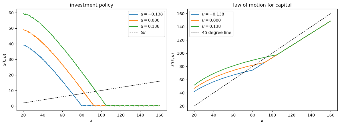
Fig. 114.1 Investment policy and law of motion#
Capital rises when \(x(k,u)\) lies above the maintenance line \(\delta k\) and falls when it lies below.
Higher demand shifts the investment policy up, so the capital stock that the industry sustains is higher when demand is strong.
114.7.1. The price of installed capital#
The planner’s problem also delivers the market value \(w\) of a unit of installed capital that appeared in (114.5).
Let \(z = x/k\) denote the investment rate.
Differentiating the Bellman equation (114.9) and using the envelope condition gives
while the first-order condition for \(x\) is
Combining them expresses the shadow price in closed form,
The marginal value of installed capital equals the current price of output plus the value of the capacity that the unit carries into the future.
Notice that (114.10) is the planner’s counterpart of the firm’s first-order condition (114.6), with \(w^* = \mathbb{E}[v_k(k',u') \mid u]\).
That correspondence is the “big \(K\), little \(k\)” logic of the lecture Rational Expectations Equilibrium in its Lucas-Prescott form.
h = lambda z, m: (1 - m.δ + z)**m.α
h_prime = lambda z, m: m.α * (1 - m.δ + z)**(m.α - 1)

z = x / m.k[:, None]
D = m.a0 + m.u[None, :] - m.a1 * m.k[:, None]
w = D + h(z, m) / h_prime(z, m) - z

# check the first-order condition (up to grid error)
Ew = np.take_along_axis(w @ m.P.T, idx, axis=0)
resid = np.abs(m.β * Ew - 1 / h_prime(z, m))
scale = np.median(1 / h_prime(z, m))
near = (m.k > 70) & (m.k < 95)          # capital levels the industry actually visits
print(f"typical size of each side of the FOC: {scale:.3f}")
print(f"median residual, all k:               {np.median(resid):.2e}")
print(f"median residual, 70 < k < 95:         {np.median(resid[near]):.2e}")
typical size of each side of the FOC: 1.396
median residual, all k:               5.35e-03
median residual, 70 < k < 95:         2.39e-03
The residual is a few tenths of one per cent of the magnitude of the terms being compared, which confirms (114.11).
It does not vanish entirely because the planner chooses \(k'\) from a finite grid, so the policy function jumps by a whole grid point at a time.
Residuals are much larger at capital levels so extreme that the industry never visits them.
114.8. Long run behavior with serially independent demand#
Lucas and Prescott next ask what happens in the long run.
They treat two cases, and the first is the special case in which \(u_t\) and \(u_s\) are independent for \(s \neq t\).
Inspecting the Bellman equation (114.9) when \(p(dz,u)\) does not depend on \(u\) shows that the optimal investment rate \(x(k,u)\) does not depend on \(u\).
A demand shift is then a pure windfall: it tells firms nothing about future demand, so it does not change investment.
Consequently the capital stock evolves deterministically, according to \(k_{t+1} = k_t h(x(k_t)/k_t)\), while output is supplied inelastically and demand shocks move only prices.
Theorem 114.2
Under independence, there are two possibilities for the capital stock.
If
and \(k_0 > 0\), then \(k_t\) converges monotonically to the unique stationary value \(k^c\) given implicitly by
Otherwise capital converges monotonically to zero.
Condition (114.13) has a familiar interpretation.
The left side is expected marginal revenue product of capital, which here is just the expected output price, because the marginal physical product is one.
The right side is a user cost of capital: a depreciation term \(\delta\) plus an interest term \(r/h'(\delta)\).
Lucas and Prescott observe that this case corresponds closely to the textbook dichotomy between short-run and long-run supply.
In the short run, capacity is fixed and demand determines price.
In the long run, demand fluctuations play no role at all: capacity is determined entirely by average demand.
Let’s verify this numerically by setting \(\rho = 0\).
m_iid = create_model(ρ=0.0)
v_iid, idx_iid, k_next_iid, x_iid = solve_model(m_iid)

# does the policy depend on u?
print("investment policy independent of u:",
      np.allclose(x_iid, x_iid[:, [0]], atol=1e-10))

# stationary capital: where x(k) crosses δ k
def stationary_k(x_col, m):
    "Capital where investment just maintains capacity."
    d = x_col - m.δ * m.k
    i = np.where(np.sign(d[:-1]) != np.sign(d[1:]))[0]
    if len(i) == 0:
        return np.nan
    i = i[0]
    return np.interp(0, [d[i+1], d[i]], [m.k[i+1], m.k[i]])

kc = stationary_k(x_iid[:, 0], m_iid)
user_cost = m_iid.δ + m_iid.r / h_prime(m_iid.δ, m_iid)
print(f"\nstationary capital k^c        = {kc:.3f}")
print(f"expected price at k^c         = {m_iid.a0 - m_iid.a1 * kc:.5f}")
print(f"user cost δ + r / h'(δ)       = {user_cost:.5f}")
investment policy independent of u: True

stationary capital k^c        = 82.807
expected price at k^c         = 0.17193
user cost δ + r / h'(δ)       = 0.17143
The stationary capital stock equates the expected price to the user cost of capital, as (114.13) requires.
Now let’s confirm that capital approaches \(k^c\) monotonically, and from either direction.
def capital_path(m, idx, k0, T=60, u_index=None):
    "Simulate capital, holding the demand state fixed if u_index is given."
    ki = np.abs(m.k - k0).argmin()
    path = np.empty(T)
    j = len(m.u) // 2 if u_index is None else u_index
    for t in range(T):
        path[t] = m.k[ki]
        ki = idx[ki, j]
    return path

fig, ax = plt.subplots(figsize=(8, 4.5))
for k0 in (30.0, 55.0, 110.0, 150.0):
    ax.plot(capital_path(m_iid, idx_iid, k0), lw=2, label=f'$k_0 = {k0:.0f}$')
ax.axhline(kc, color='k', ls='--', lw=1, label='$k^c$')
ax.set_xlabel('$t$'); ax.set_ylabel('$k_t$')
ax.legend()
plt.tight_layout()
plt.show()
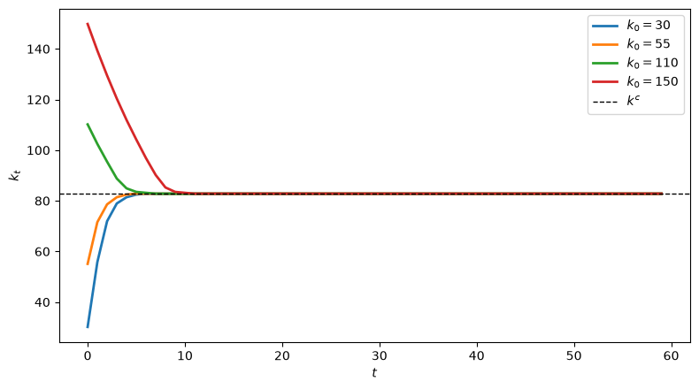
Fig. 114.2 Capital paths under IID demand#
Convergence is monotone and the limit does not depend on the initial capital stock.
114.9. Long run behavior with serially correlated demand#
The more interesting case allows demand shifts to be positively serially correlated, so that a high demand today signals high demand tomorrow.
Now the current demand state does affect investment, and the capital stock is genuinely stochastic.
To characterize the long run, Lucas and Prescott impose additional restrictions on the \(\{u_t\}\) process, whose purpose is to guarantee that the distribution of \((k_t, u_t)\) settles down.
In words, they assume that
from any current \(u\), next period’s shock lands in any non-degenerate interval with positive probability
\(u_t\) has a limiting distribution that does not depend on the initial \(u_0\) and that puts positive probability on every non-degenerate interval
\(\mathbb{P}\{u_{t+1} \geq x \mid u_t\}\) is strictly increasing in \(u_t\), so high demand today always signals high demand tomorrow
consumer surplus \(s(k,u)\) converges uniformly as \(u \to \pm\infty\)
A Gaussian AR(1) process with \(0 < \rho < 1\) satisfies these conditions, which is the example they give and the one we simulate.
The analysis then proceeds by bounding the capital stock.
Let \(\bar v(k)\) and \(\underline v(k)\) be the limits of the expected value function as \(u \to \infty\) and \(u \to -\infty\), and let \(\bar x(k)\) and \(\underline x(k)\) be the associated investment policies.
Because investment is increasing in \(u\), these bracket the policy for every \(u\).
Let \(\bar k\) solve \(\bar x(k) = \delta k\) and let \(\underline k\) solve \(\underline x(k) = \delta k\).
These are the capital stocks that would be sustained under permanently maximal and permanently minimal demand.
Lucas and Prescott then prove that
the sets \((0, \underline k)\) and \((\bar k, \infty)\), paired with any demand state, are transient: once the industry leaves them it does not return, and from any starting point it enters \((\underline k, \bar k)\) with probability approaching one
the set \(B = (\underline k, \bar k) \times E\), where \(E\) is the set of possible values of \(u\), is a single ergodic set
Theorem 114.3
If \(B\) is non-empty, then for all \((k,u)\) and every initial state \((k_0, u_0)\),
exists and does not depend on \((k_0, u_0)\).
The function \(P\) is a probability distribution that assigns probability zero to the transient sets and positive probability to every subset of \(B\) with positive area.
Theorem 114.4
If \(B\) is non-empty, then for any initial state, with probability one
where \(k^*\) is the mean of \(k\) under the invariant distribution \(P\).
The ergodic set is non-empty – and so this long-run behavior applies – if and only if
which says that demand must sometimes be strong enough to justify holding any capital at all.
Theorem 114.3 and Theorem 114.4 are the results that make this model an object that econometricians can use.
The first says that the model implies a well-defined stationary probability distribution for the observable time series.
The second says that sample averages computed from a single long realization converge to the corresponding population moments of that distribution.
Let’s compute the bounds \(\underline k\) and \(\bar k\) for our parameterization and check that simulations behave as the theorems say.
bounds = np.array([stationary_k(x[:, j], m) for j in range(len(m.u))])
k_lo_star, k_hi_star = bounds.min(), bounds.max()
print(f"conditional stationary capital, lowest demand state:  {k_lo_star:.2f}")
print(f"conditional stationary capital, highest demand state: {k_hi_star:.2f}")
print(f"ergodic set for capital: ({k_lo_star:.2f}, {k_hi_star:.2f})")
conditional stationary capital, lowest demand state:  71.23
conditional stationary capital, highest demand state: 94.39
ergodic set for capital: (71.23, 94.39)
Now we simulate the equilibrium Markov process from two very different initial capital stocks, using the same sequence of demand shocks.
def simulate(m, idx, k0, T=20_000, seed=0):
    "Simulate the equilibrium Markov process for (k, u)."
    mc = qe.MarkovChain(m.P, m.u)
    u_idx = mc.simulate_indices(T, init=len(m.u)//2, random_state=seed)
    ki = np.abs(m.k - k0).argmin()
    k_path = np.empty(T)
    for t in range(T):
        k_path[t] = m.k[ki]
        ki = idx[ki, u_idx[t]]
    p_path = m.a0 + m.u[u_idx] - m.a1 * k_path
    return k_path, p_path

k_low, p_low = simulate(m, idx, k0=30.0, seed=1)
k_high, p_high = simulate(m, idx, k0=150.0, seed=1)

fig, ax = plt.subplots(figsize=(9, 4.5))
ax.plot(k_low[:250], lw=2, label='$k_0 = 30$')
ax.plot(k_high[:250], lw=2, label='$k_0 = 150$')
ax.axhline(k_lo_star, color='k', ls='--', lw=1)
ax.axhline(k_hi_star, color='k', ls='--', lw=1, label='ergodic set')
ax.set_xlabel('$t$'); ax.set_ylabel('$k_t$')
ax.legend()
plt.tight_layout()
plt.show()
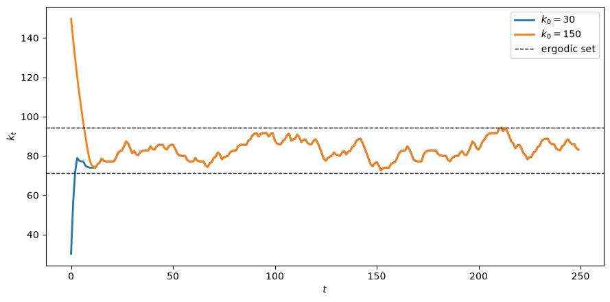
Fig. 114.3 Capital paths entering the ergodic set#
Both paths are drawn into the ergodic set and then fluctuate inside it forever.
The next figure compares the long-run distributions of capital computed from the two simulations, after discarding a burn-in sample.
burn = 2000
fig, axes = plt.subplots(1, 2, figsize=(12, 4.5))

axes[0].hist(k_low[burn:], bins=60, density=True, alpha=0.5, label='from $k_0 = 30$')
axes[0].hist(k_high[burn:], bins=60, density=True, alpha=0.5, label='from $k_0 = 150$')
axes[0].set_xlabel('$k$'); axes[0].set_ylabel('density')
axes[0].set_title('invariant distribution of capital')
axes[0].legend()

axes[1].hist(p_low[burn:], bins=60, density=True, alpha=0.5)
axes[1].set_xlabel('$p$'); axes[1].set_ylabel('density')
axes[1].set_title('invariant distribution of price')

plt.tight_layout()
plt.show()

print(f"mean capital from k_0 = 30:  {k_low[burn:].mean():.3f}")
print(f"mean capital from k_0 = 150: {k_high[burn:].mean():.3f}")
print(f"range visited: ({k_low[burn:].min():.2f}, {k_low[burn:].max():.2f})")
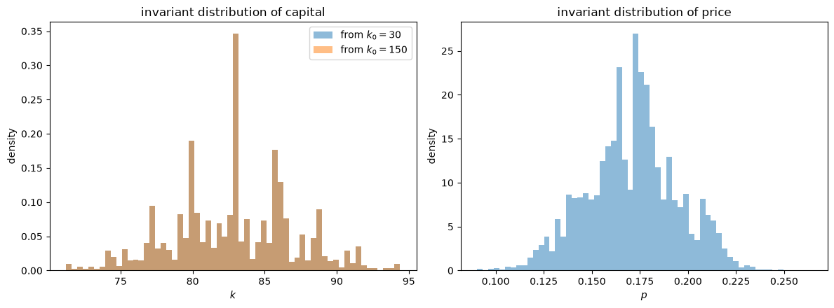
Fig. 114.4 Invariant distributions of capital and price#
mean capital from k_0 = 30:  82.792
mean capital from k_0 = 150: 82.792
range visited: (71.23, 94.39)
The two histograms coincide, as Theorem 114.3 promises, and the capital stock stays inside the ergodic set.
Finally, here is Theorem 114.4 in action: time averages from a single realization converge to the mean of the invariant distribution.
running_mean = np.cumsum(k_low) / np.arange(1, len(k_low) + 1)

fig, ax = plt.subplots(figsize=(8, 4.5))
ax.plot(running_mean, lw=2)
ax.axhline(k_low[burn:].mean(), color='k', ls='--', lw=1, label='$k^*$')
ax.set_xlabel('$T$'); ax.set_ylabel(r'$T^{-1}\sum_{t \leq T} k_t$')
ax.set_xscale('log')
ax.legend()
plt.tight_layout()
plt.show()
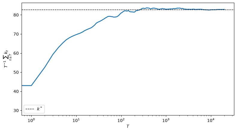
Fig. 114.5 Time average of capital#
114.10. Relation to the rational expectations lecture#
It is worth collecting the correspondences between this lecture and Rational Expectations Equilibrium.
this lecture |
||
|---|---|---|
uncertainty |
none |
Markov demand shifter \(u_t\) |
adjustment costs |
quadratic, \(\gamma (y'-y)^2/2\) |
concave technology \(k' = k h(x/k)\) |
equilibrium object |
belief \(H\) with \(Y' = H(Y)\) |
price process \(\{p_t\}\), equivalently policy \(x(k,u)\) |
equilibrium concept |
\(H\) is a fixed point of \(\Phi\) |
anticipated price distribution equals actual |
how it is computed |
planning problem, solved as an LQ problem |
planning problem, solved by dynamic programming |
what the planner maximizes |
consumer plus producer surplus |
discounted consumer surplus (114.8) |
equilibrium dynamics |
\(Y_{t+1} = \kappa_0 + \kappa_1 Y_t\) |
Markov process for \((k_t, u_t)\) |
long-run behavior |
convergence to a steady state |
convergence to an invariant distribution |
The deepest common element is the strategy for computing an equilibrium.
In both lectures, the direct approach – guess a law of motion, compute the induced best response, and iterate – is unreliable, because that mapping need not be a contraction.
In both lectures, the remedy is to find a planning problem whose Euler equations coincide with the equilibrium conditions, and then to solve the planning problem by dynamic programming.
The lecture Rational Expectations Equilibrium verifies this correspondence by matching Euler equations for a particular linear-quadratic example.
Theorem 114.1 is the general statement: for this class of economies, the set of competitive equilibria and the set of solutions of the planning problem coincide, and both are singletons.
What the baby version cannot show, because it has no uncertainty, is the payoff that Lucas and Prescott were after: an equilibrium that is a stationary stochastic process, with an invariant distribution and ergodic time averages.
That is what makes it possible to confront such a model with data, and what led on to rational expectations econometrics.
The companion lecture Optimal Growth Under Uncertainty and Tobin’s q pursues exactly this theme in a one-sector growth model.
Brock and Mirman [1972] prove there the counterparts of Theorem 114.3 and Theorem 114.4: the distribution of capital converges to an invariant distribution that does not depend on initial conditions, and time averages along a single realization converge to population moments.
That lecture also shows what the shadow price of capital in such a planning problem becomes in a competitive equilibrium – namely Tobin’s \(q\) – and examines a subtle question about the differentiability of the value function that the answer depends on.
114.11. Exercises#
Exercise 114.1
The user cost of capital in (114.13) depends on the curvature parameter \(\alpha\) of the adjustment technology through \(h'(\delta) = \alpha\).
Explain why a lower \(\alpha\) – meaning stronger adjustment costs – should reduce the long-run capital stock.
For the serially independent case, compute the stationary capital stock \(k^c\) for \(\alpha \in \{0.4, 0.6, 0.8, 1.0\}\) and verify in each case that the marginal condition (114.13) holds.
Confirm that when \(\alpha = 1\) the accumulation equation is \(k_{t+1} = (1-\delta)k_t + x_t\) and the user cost is the textbook \(\delta + r\).
Solution
A lower \(\alpha\) makes \(h\) more concave, so a unit of investment buys less capacity at the margin.
Since \(h'(\delta) = \alpha\), the interest component of the user cost, \(r / h'(\delta) = r/\alpha\), rises as \(\alpha\) falls.
A higher user cost must be matched by a higher expected price, and since demand slopes down, that means a smaller capital stock.
print(f"{'α':>5} {'k^c':>10} {'E[price]':>12} {'user cost':>12}")
for α in (0.4, 0.6, 0.8, 1.0):
    m_α = create_model(ρ=0.0, α=α, k_lo=5.0, k_hi=160.0, n_k=600)
    _, _, _, x_α = solve_model(m_α)
    kc_α = stationary_k(x_α[:, 0], m_α)
    price = m_α.a0 - m_α.a1 * kc_α
    cost = m_α.δ + m_α.r / h_prime(m_α.δ, m_α)
    print(f"{α:>5.1f} {kc_α:>10.3f} {price:>12.5f} {cost:>12.5f}")
    α        k^c     E[price]    user cost
  0.4     77.454      0.22546      0.22500
  0.6     81.594      0.18406      0.18333
  0.8     83.664      0.16336      0.16250
  1.0     84.958      0.15042      0.15000
Stronger adjustment costs (lower \(\alpha\)) do indeed lower the long-run capital stock.
With \(\alpha = 1\) we have \(h(z) = 1 - \delta + z\), so \(k' = k(1 - \delta + x/k) = (1-\delta)k + x\), and \(h'(\delta) = 1\), so the user cost is \(\delta + r\).
Exercise 114.2
Theorem 114.1 says that the planner’s policy is the competitive equilibrium.
Verify this numerically, using the “big \(K\), little \(k\)” logic of Rational Expectations Equilibrium.
Solve the problem of an individual price-taking firm that
owns capital \(k_i\) and chooses \(k_i'\) subject to the same accumulation technology
takes as given the aggregate capital stock \(K\), which evolves according to the planner’s policy computed above
takes as given the price \(p = a_0 + u - a_1 K\), which depends on aggregate, not own, capital
Then check that when the firm’s own capital equals aggregate capital, \(k_i = K\), the firm chooses exactly what the planner chooses.
Use a coarser grid for the firm’s own capital to keep the computation small.
Solution
The firm’s Bellman equation is
where \(K' \) follows the planner’s law of motion.
Note that the firm’s own capital affects its revenue but not the price.
def firm_problem(m, idx_agg, n_i=80, tol=1e-8, maxit=1000, howard=20):
    "Solve an individual firm's problem taking the aggregate law of motion as given."
    sub = np.linspace(0, len(m.k) - 1, n_i).astype(int)   # firm grid ⊂ aggregate grid
    ki = m.k[sub]
    n_K, n_u = len(m.k), len(m.u)

    Xi = ki[:, None] * ((ki[None, :] / ki[:, None])**(1/m.α) - (1 - m.δ))
    Ri = np.where(Xi >= 0, -Xi, -1e12)                    # (k_i, k_i')
    price = m.a0 + m.u[None, :] - m.a1 * m.k[:, None]     # (K, u)
    revenue = ki[:, None, None] * price[None, :, :]       # (k_i, K, u)

    v_i = np.zeros((n_i, n_K, n_u))
    u_cols = np.arange(n_u)[None, :]
    for it in range(maxit):
        EV = np.tensordot(v_i, m.P, axes=([2], [1]))      # E[v_i(k_i', K', u') | u]
        cont = EV[:, idx_agg, u_cols]                     # impose K' = planner's choice
        obj = Ri[:, :, None, None] + m.β * cont[None, :, :, :]
        pol = obj.argmax(axis=1)
        v_new = revenue + np.take_along_axis(obj, pol[:, None, :, :], axis=1)[:, 0, :, :]

        for _ in range(howard):
            EV = np.tensordot(v_new, m.P, axes=([2], [1]))
            cont = EV[:, idx_agg, u_cols]
            v_new = (revenue + Ri[np.arange(n_i)[:, None, None], pol]
                     + m.β * np.take_along_axis(cont, pol, axis=0))

        if np.max(np.abs(v_new - v_i)) < tol:
            v_i = v_new
            break
        v_i = v_new

    return ki, sub, pol

ki, sub, pol_firm = firm_problem(m, idx)

# compare the firm's choice with the planner's, evaluated at k_i = K
gaps = []
for a, K_i in enumerate(sub):
    for j in range(len(m.u)):
        gaps.append(abs(ki[pol_firm[a, K_i, j]] - m.k[idx[K_i, j]]))
gaps = np.array(gaps)

print(f"firm grid spacing:                   {np.diff(ki).mean():.3f}")
print(f"mean |firm choice - planner choice|: {gaps.mean():.3f}")
print(f"max  |firm choice - planner choice|: {gaps.max():.3f}")
firm grid spacing:                   1.772
mean |firm choice - planner choice|: 0.590
max  |firm choice - planner choice|: 1.404
The discrepancies are smaller than the spacing of the firm’s own capital grid.
So the price-taking firm, responding optimally to the price process that the planner’s allocation generates, chooses to do exactly what the planner does.
That is the content of Theorem 114.1, and it is the Lucas-Prescott counterpart of the fixed point condition \(H(Y) = h(Y,Y)\) in Rational Expectations Equilibrium.
Exercise 114.3
Theorem 114.3 says that the invariant distribution does not depend on initial conditions, but it says nothing about how wide that distribution is.
Investigate how serial correlation in demand affects the ergodic set.
For \(\rho \in \{0.0, 0.5, 0.9, 0.98\}\), compute the ergodic bounds \(\underline k\) and \(\bar k\).
Simulate each economy and compare the invariant distributions of capital.
Explain the pattern. Why does the \(\rho = 0\) case produce a degenerate distribution for capital?
Solution
Here is one solution.
fig, ax = plt.subplots(figsize=(9, 4.5))
print(f"{'ρ':>6} {'k_lo':>9} {'k_hi':>9} {'width':>9} {'std(k)':>9}")

for ρ in (0.0, 0.5, 0.9, 0.98):
    m_ρ = create_model(ρ=ρ)
    _, idx_ρ, _, x_ρ = solve_model(m_ρ)
    b = np.array([stationary_k(x_ρ[:, j], m_ρ) for j in range(len(m_ρ.u))])
    k_ρ, _ = simulate(m_ρ, idx_ρ, k0=80.0, seed=3)
    print(f"{ρ:>6.2f} {b.min():>9.2f} {b.max():>9.2f} "
          f"{b.max()-b.min():>9.2f} {k_ρ[2000:].std():>9.3f}")
    if ρ > 0:      # the ρ = 0 distribution is a spike at k^c, so we omit it here
        ax.hist(k_ρ[2000:], bins=50, density=True, alpha=0.45, label=f'$\\rho = {ρ}$')

ax.set_xlabel('$k$'); ax.set_ylabel('density')
ax.legend()
plt.tight_layout()
plt.show()
     ρ      k_lo      k_hi     width    std(k)
  0.00     82.81     82.81      0.00     0.000
  0.50     80.00     85.61      5.61     0.797
  0.90     71.23     94.39     23.16     4.156
  0.98     53.33    112.28     58.95    13.552
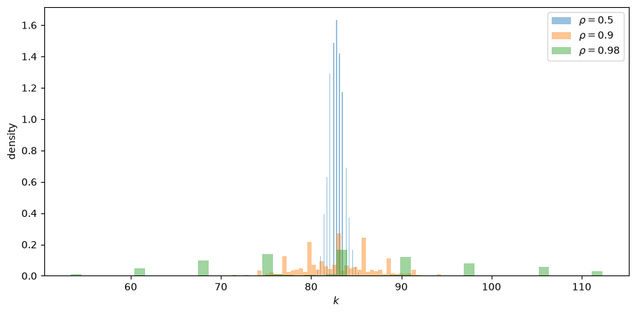
The more persistent is demand, the wider the ergodic set and the more dispersed the invariant distribution of capital.
(The figure omits \(\rho = 0\), whose distribution is a spike at \(k^c\) that would dwarf the others.)
The reason is the one Lucas and Prescott emphasize.
Investment responds to news about future demand, not to current demand as such.
When \(\rho = 0\), a demand shift conveys no information about the future, so investment does not respond at all, and capital converges to the single deterministic value \(k^c\) of Theorem 114.2: the invariant distribution of capital is degenerate even though prices keep fluctuating.
As \(\rho\) rises, a high demand state signals a sustained period of high prices, so firms invest more, and the capital stock inherits the persistence of demand.