115. Optimal Growth Under Uncertainty and Tobin’s q#
115.1. Overview#
This lecture studies two papers.
The first is Brock and Mirman [1972], a classic analysis of optimal one-sector growth when the production function is hit by random shocks.
The second is Sargent [1980], which adds one small ingredient – irreversible investment – and uses the result to think about James Tobin’s \(q\) theory of investment.
The lecture Investment Under Uncertainty studied a competitive industry whose equilibrium is the solution of a planning problem, and whose equilibrium is a Markov process with an invariant distribution.
Brock and Mirman ask the same questions about a one-sector growth model:
does the planning problem have a well-behaved solution, with continuous and monotone policy functions?
the optimal policy makes capital a Markov process; does that process have an invariant distribution?
does the distribution of capital converge to it from any initial condition?
do time averages computed from a single realization converge to population moments?
The last two questions are the reason both papers matter for econometrics.
A model that answers them affirmatively delivers a stationary, ergodic stochastic process for observable time series.
Sample moments computed from one long realization then estimate population moments, which is exactly what the rational expectations econometrics of Hansen and Sargent [1980] requires.
Sargent [1980] puts the Brock-Mirman apparatus to work on a question in macroeconomics: when, and in what sense, is there an investment demand schedule relating investment to Tobin’s \(q\)?
Along the way, this lecture pauses over a technical issue that turns out to be central:
the derivative of the planner’s value function with respect to capital is the competitive price of used capital, i.e. it is essentially Tobin’s \(q\)
so the analysis stands or falls on whether that derivative exists
irreversible investment creates a corner, and at a corner the standard argument for differentiability breaks down
We’ll describe the difficulty, note a gap in the published argument, and give a corrected proof.
Let’s start with some imports:
import numpy as np
import matplotlib.pyplot as plt
from collections import namedtuple
115.2. The Brock-Mirman planning problem#
A planner chooses consumption to maximize
subject to
where \(k_t\) is capital per worker, \(i_t\) is investment, and \(\{r_t\}\) is a sequence of independent and identically distributed shocks to production.
Brock and Mirman assume that for each realization of the shock, \(f(\cdot, r)\) is increasing, strictly concave, and satisfies the Inada conditions
and that \(f\) is increasing in \(r\), so that a higher shock means more output.
The period utility function \(u\) is increasing, strictly concave, and differentiable.
In their formulation capital depreciates fully in one period, so that \(k_{t+1} = i_t\) and current resources are \(s_t = f(k_{t-1}, r_{t-1})\).
The Bellman equation is
where \(\nu\) is the distribution of the shock.
Standard arguments – a contraction mapping, plus preservation of monotonicity and concavity – give a unique bounded solution \(v\), attained by a unique consumption policy \(c = g(s)\) and investment policy \(x = h(s) = s - g(s)\).
Proposition 115.1
The optimal policies \(g\) and \(h\) are increasing and continuous, with \(g(0) = h(0) = 0\).
Brock and Mirman prove monotonicity from the first-order condition
which is the stochastic analogue of the Euler equation.
If \(g\) did not increase with \(s\), the left side of (115.3) would stay constant while the right side would fall, because \(f\) increases and \(u'\) and \(f'\) decrease.
115.3. Long-run behavior#
The optimal policy makes capital a Markov process,
and Brock and Mirman devote most of their paper to the long-run behavior of this process.
The strategy resembles the one used in Investment Under Uncertainty.
Consider the deterministic difference equations obtained by fixing the shock at its lowest possible value \(\underline r\) and at its highest possible value \(\bar r\):
Let \(\underline k\) be a positive fixed point of the first and \(\bar k\) a positive fixed point of the second.
Because \(f\) is increasing in the shock and \(h\) is increasing, \(\underline k \leq \bar k\).
Brock and Mirman say that the model has a stable configuration of fixed points when \(\underline k\) and \(\bar k\) are positive and \(\underline k < \bar k\).
They then show that
the sets of capital stocks below \(\underline k\) and above \(\bar k\) are transient: the process leaves them and does not return
the interval \([\underline k, \bar k]\) is where the process eventually lives
Theorem 115.1
There is a distribution function \(F\) such that the distribution \(F_t\) of \(k_t\) converges to \(F\) uniformly, and \(F\) does not depend on the initial capital stock.
Theorem 115.1 is the counterpart of the invariant-distribution theorem of Investment Under Uncertainty.
An important part of the proof is an argument about the inverse optimal process, which runs the Markov process backwards in time; Brock and Mirman use it to show that a stationary distribution exists and is unique without appealing to heavier machinery from probability theory.
Convergence of distributions is not by itself enough for econometrics.
What an econometrician needs in addition is a mean-ergodic theorem: a guarantee that averages computed along a single realization converge to moments of \(F\),
For Markov processes with a unique invariant distribution and a stable configuration of fixed points, such laws of large numbers are available; Sargent [1980] invokes the version in Doob’s book to justify computing population moments of his model and comparing them with sample moments.
This is the bridge from Brock and Mirman’s theory to the rational expectations econometrics developed in the late 1970s and early 1980s.
Without Theorem 115.1 and (115.5), a likelihood function computed from a single time series would have no firm justification.
Note
Brock and Mirman [1972] study the case in which the shocks are independent and identically distributed.
The lecture Investment Under Uncertainty describes a parallel set of results for a model in which the shock is serially correlated.
In both cases the economics is the same: the state must eventually wander inside a compact set on which the process is well behaved, and the boundaries of that set are the stationary points associated with the most and least favorable shocks.
115.4. Irreversible investment and Tobin’s q#
Sargent [1980] modifies the model in one respect: capital, once installed, cannot be eaten.
Output can be consumed or added to the capital stock, but the conversion does not run backwards,
where \(0 < \delta < 1\) is the depreciation rate.
Production is \(y_t = f(K_t)\theta_t\), and the one-period utility function \(u(c_t, e_t)\) is hit by a preference shock \(e_t\).
The shocks \((\theta_t, e_t)\) are independent and identically distributed over time.
Why does this small change matter?
In the model with reversible investment, the price of a unit of installed capital always equals the price of a unit of newly produced output, so Tobin’s \(q\) is identically one and firms have no investment demand schedule at all.
The irreversibility constraint is a friction that lets the price of installed capital fall below the price of new capital.
Sargent describes a competitive economy in which households own capital, rent it to firms, and trade claims to installed capital at a relative price \(p_{Kt}\), which is Tobin’s \(q\).
Following Lucas and Prescott [1971] – exactly the strategy of Investment Under Uncertainty – he studies the competitive equilibrium indirectly, through the planning problem that generates it.
The planner solves
Let \(\lambda \geq 0\) be the multiplier on the irreversibility constraint.
The first-order condition is
and the price of installed capital is
So this model implies
\(q \leq 1\) always
\(q = 1\) exactly when investment is positive
\(q < 1\) exactly when the irreversibility constraint binds, which is when investment is zero
Notice what (115.9) says: Tobin’s \(q\) is the derivative of the planner’s value function, normalized by marginal utility.
Everything therefore depends on whether \(v_K\) exists.
115.5. Differentiability of the value function#
Here is the difficulty.
The standard tool for differentiability of a value function is the theorem of Benveniste and Scheinkman [1979].
Theorem 115.2 (Benveniste-Scheinkman)
Let \(v\) be concave on an open set \(D\) and let \(K_0 \in D\).
Suppose \(W\) is concave, differentiable at \(K_0\), and satisfies \(W(K) \leq v(K)\) on a neighborhood of \(K_0\), with \(W(K_0) = v(K_0)\).
Then \(v\) is differentiable at \(K_0\) and \(v'(K_0) = W'(K_0)\).
The usual way to build such a \(W\) is to take the optimal plan at \(K_0\), freeze next period’s capital at its optimal value \(K_0'\), and let consumption absorb the change in \(K\):
This is a feasible plan, so \(W_1 \leq v\), with equality at \(K_0\), and it is differentiable.
But feasibility requires \(K_0' \geq (1-\delta)K\), that is \(K \leq K_0'/(1-\delta)\).
When investment is positive, \(K_0' > (1-\delta)K_0\) and the plan is feasible on a full neighborhood of \(K_0\).
When investment is zero, \(K_0' = (1-\delta)K_0\) exactly, and the plan is infeasible for every \(K > K_0\).
At a corner, the standard support function is available only from the left.
This is precisely where the published argument becomes delicate, and in our reading it has gaps.
Note
Two specific difficulties.
First, Sargent [1980] states the derivative of the value function in the form
which is obtained by substituting the first-order condition (115.8) with equality into the envelope condition.
That substitution is legitimate only where investment is positive.
Where investment is zero, \(\lambda > 0\) and the formula overstates \(v_K\); the paper’s own subsequent inequality records this, so the two statements are not consistent with each other.
Second, the argument establishes differentiability of the value function by induction along the iterates \(v^j = T^j v^0\), and then passes to the limit.
That route requires knowing how the set of capital stocks at which the constraint just binds is structured.
The published proof handles three configurations, drawn in its Figures 3-5, and appeals to an appendix that assumes the iterates are twice differentiable almost everywhere.
The appendix in turn justifies this by differentiating the first-order condition and observing that “since the right-hand side exists almost everywhere, so does the left,” which does not follow as stated, and it asserts without proof that the set of binding points has Lebesgue measure zero.
Fortunately the conclusion is true, and there is a route to it that avoids the induction on iterates entirely.
The key observation is that at a corner a different feasible plan supplies the needed support function: investing nothing is feasible at every capital stock, so it works on both sides.
Proposition 115.2
Assume \(u\) and \(f\) are increasing, strictly concave and continuously differentiable, with \(u_c(0,e) = \infty\) and \(f'(0) = \infty\).
Then for each \((\theta, e)\) the value function \(v(\cdot,\theta,e)\) defined by (115.7) is continuously differentiable on \((0,\infty)\), and
where \(c\) and \(K'\) are optimal at \((K,\theta,e)\).
Where investment is positive, (115.11) reduces to \(v_K = u_c(c,e)[f'(K)\theta + (1-\delta)]\).
Where investment is zero, \(v_K < u_c(c,e)[f'(K)\theta + (1-\delta)]\).
Proof. Step 0. The operator associated with (115.7) maps bounded continuous concave functions into bounded continuous strictly concave functions, so \(v(\cdot,\theta,e)\) is concave and continuous, and the optimal policy is single valued and continuous.
Step 1 (investment positive). Suppose \(I(K_0,\theta,e) > 0\), and let \(K_0'\) be the optimal choice.
Then \(K_0' > (1-\delta)K_0\), so by continuity the plan that freezes next period’s capital at \(K_0'\) is feasible for all \(K\) in a neighborhood of \(K_0\).
The function \(W_1\) of (115.10) is therefore concave, continuously differentiable, dominated by \(v\), and equal to \(v\) at \(K_0\).
Theorem 115.2 gives differentiability at \(K_0\) with
Because the first-order condition holds with equality here, \(\beta \mathbb{E}[v_K(K_0',\cdot)] = u_c(c,e)\), and substituting gives (115.11).
Step 2 (investment zero, conditional on a smaller capital stock). Suppose \(I(K_0,\theta,e) = 0\), so that \(K_0' = (1-\delta)K_0\) and investing nothing is optimal at \(K_0\).
Consider instead the plan that invests nothing this period and behaves optimally thereafter:
Investing nothing is feasible at every capital stock, so \(W_2 \leq v\) everywhere, with \(W_2(K_0) = v(K_0)\), and \(W_2\) is concave.
Suppose that \(v(\cdot,\theta',e')\) is differentiable at \((1-\delta)K_0\) for every \((\theta',e')\).
Then \(W_2\) is differentiable at \(K_0\); differentiation under the expectation is legitimate because the functions \(v(\cdot,\theta',e')\) are concave, hence locally Lipschitz with a common bound on a compact neighborhood.
Theorem 115.2 then gives differentiability of \(v\) at \(K_0\), with
which is (115.11).
Step 3 (a region where the corner cannot bind). Because \(f'(0) = \infty\), there is an \(\eta > 0\) such that \(I(K,\theta,e) > 0\) for every \(K \leq \eta\) and every \((\theta,e)\).
The intuition is that the marginal product of capital becomes arbitrarily large as capital approaches zero, so that giving up a little consumption today buys a great deal of consumption tomorrow.
Making this precise requires comparing the rates at which the two sides of (115.8) diverge as \(K \downarrow 0\), since with, say, logarithmic utility both sides become unbounded.
Sargent [1980] proves the statement in his Appendix A (his Proposition A2), under an explicit restriction on \(u\) and \(f\) that he imposes for this purpose.
That result is the one ingredient of his appendix that the argument below borrows, and it is independent of the differentiability question at issue here.
By Step 1, \(v(\cdot,\theta,e)\) is therefore differentiable on \((0,\eta]\) for every \((\theta,e)\).
Step 4 (bootstrap). Let
We claim that if \((0, A) \subseteq D\) then \((0, A/(1-\delta)) \subseteq D\).
Take \(K < A/(1-\delta)\) and any \((\theta,e)\).
If \(I(K,\theta,e) > 0\), Step 1 applies directly.
If \(I(K,\theta,e) = 0\), then \((1-\delta)K < A\), so \(v(\cdot,\theta',e')\) is differentiable at \((1-\delta)K\) for every \((\theta',e')\), and Step 2 applies.
By Step 3 we may start the induction at \(A = \eta\).
Since \(1/(1-\delta) > 1\), iterating the claim gives \((0, \eta (1-\delta)^{-n}) \subseteq D\) for every \(n\), and therefore \(D = (0,\infty)\).
Step 5 (continuity). A concave function that is differentiable on an open interval has a continuous derivative there, so \(v(\cdot,\theta,e)\) is continuously differentiable.
Finally, where investment is zero the first-order condition holds with \(\lambda > 0\), so \(\beta \mathbb{E}[v_K(K',\cdot)] < u_c\), and (115.11) gives \(v_K < u_c[f'(K)\theta + (1-\delta)]\).
The corrected formula has a natural reading.
Iterating (115.11) forward gives
A marginal unit of capital installed today yields marginal products for as long as it survives, and each is valued at the marginal utility of consumption on the date it arrives.
When investment is positive, the market prices that whole stream at the cost of a unit of new output, and (115.12) collapses to \(u_c[f'(K)\theta + (1-\delta)]\).
When investment is zero, it does not, and the difference is exactly what pushes \(q\) below one.
115.6. Computing the model#
We now solve the model of (115.7) with
The shocks \(\theta\) and \(e\) each take two values with equal probability and are independent of each other and over time.
One numerical detail matters a great deal.
The irreversibility constraint says \(K' \geq (1-\delta)K\), so we want \((1-\delta)K\) to be a point of the capital grid whenever \(K\) is.
Following Sargent [1980], we use a geometric grid with ratio \((1-\delta)^{1/z}\) for an integer \(z\), so that \((1-\delta)K_i = K_{i-z}\) exactly.
Model = namedtuple("Model", "β δ a z K θ e W nθ ne")

def create_model(β=0.95, δ=0.05, a=0.25, z=10, n_K=500, K_hi=20.0,
                 θ_vals=(0.85, 1.15), e_vals=(0.6, 1.4)):
    "Geometric capital grid so that (1-δ)K is itself a grid point."
    ratio = (1 - δ)**(1/z)
    K = K_hi * ratio**np.arange(n_K - 1, -1, -1)
    θ, e = np.array(θ_vals), np.array(e_vals)
    W = np.outer(np.ones(len(θ))/len(θ), np.ones(len(e))/len(e))
    return Model(β, δ, a, z, K, θ, e, W, len(θ), len(e))

f  = lambda m, K: K**m.a
f_prime = lambda m, K: m.a * K**(m.a - 1)
The planner chooses next period’s capital from the grid, subject to positive consumption and to irreversibility.
def solve_model(m, irreversible=True, tol=1e-10, maxit=5000, howard=50):
    "Value function iteration with Howard policy improvement steps."
    nK = len(m.K)
    C = f(m, m.K)[:, None] * m.θ[None, :]                       # output (K, θ)
    C = C[:, None, :] + (1 - m.δ)*m.K[:, None, None] - m.K[None, :, None]
    ok = C > 1e-12                                              # (K, K', θ)

    if irreversible:                                            # K' ≥ (1-δ)K
        irr = np.zeros((nK, nK), bool)
        for i in range(nK):
            irr[i, max(i - m.z, 0):] = True
        ok = ok & irr[:, :, None]

    U = np.where(ok[:, :, :, None],
                 m.e[None, None, None, :] * np.log(np.where(ok, C, 1.0))[:, :, :, None],
                 -1e12)

    v = np.zeros((nK, m.nθ, m.ne))
    for it in range(maxit):
        EV = np.tensordot(v, m.W, axes=([1, 2], [0, 1]))        # E v(K') over (θ', e')
        obj = U + m.β * EV[None, :, None, None]
        idx = obj.argmax(axis=1)
        v_new = np.take_along_axis(obj, idx[:, None, :, :], axis=1)[:, 0, :, :]

        for _ in range(howard):
            EV = np.tensordot(v_new, m.W, axes=([1, 2], [0, 1]))
            v_new = (np.take_along_axis(U, idx[:, None, :, :], axis=1)[:, 0, :, :]
                     + m.β * EV[idx])

        if np.max(np.abs(v_new - v)) < tol:
            v = v_new
            break
        v = v_new

    K_next = m.K[idx]
    I = K_next - (1 - m.δ) * m.K[:, None, None]
    C_pol = (f(m, m.K)[:, None, None] * m.θ[None, :, None]
             + (1 - m.δ) * m.K[:, None, None] - K_next)
    return v, idx, K_next, I, C_pol
To compute \(q\) we need \(v_K\), and Proposition 115.2 tells us how to get it: equation (115.11) is a linear fixed point problem in \(v_K\) given the optimal policy, and it is a contraction with modulus \(\beta(1-\delta)\).
def marginal_value(m, idx, C_pol, tol=1e-13, maxit=50_000):
    "Solve the envelope equation v_K = u_c f'(K)θ + β(1-δ) E v_K(K')."
    vK = np.zeros_like(C_pol)
    direct = (m.e[None, None, :]/C_pol) * f_prime(m, m.K)[:, None, None] * m.θ[None, :, None]
    for _ in range(maxit):
        EvK = np.tensordot(vK, m.W, axes=([1, 2], [0, 1]))
        new = direct + m.β * (1 - m.δ) * EvK[idx]
        if np.max(np.abs(new - vK)) < tol:
            return new
        vK = new
    return vK

m = create_model()
v, idx, K_next, I, C_pol = solve_model(m)
vK = marginal_value(m, idx, C_pol)

u_c = m.e[None, None, :] / C_pol
E_vK = np.tensordot(vK, m.W, axes=([1, 2], [0, 1]))
q = m.β * E_vK[idx] / u_c
corner = I <= 1e-12

print(f"share of states with zero investment: {corner.mean():.3f}")
share of states with zero investment: 0.567
Let’s check Proposition 115.2 numerically, by comparing the envelope formula with a finite-difference derivative of the computed value function.
vK_fd = np.gradient(v, m.K, axis=0)
naive = u_c * (f_prime(m, m.K)[:, None, None] * m.θ[None, :, None] + (1 - m.δ))
mid = ((m.K > 2.2) & (m.K < 7.0))[:, None, None] & np.ones_like(corner)

rel = lambda x: np.median((np.abs(x - vK_fd)/np.abs(vK_fd))[mid & sel])

sel = ~corner
print(f"investment positive: envelope error {rel(vK):.4f}, "
      f"naive formula error {rel(naive):.4f}")
sel = corner
print(f"investment zero:     envelope error {rel(vK):.4f}, "
      f"naive formula error {rel(naive):.4f}")
investment positive: envelope error 0.0005, naive formula error 0.0066
investment zero:     envelope error 0.0001, naive formula error 0.3856
Where investment is positive, both formulas agree with the numerical derivative.
Where investment is zero, the envelope formula (115.11) remains accurate while the formula \(u_c[f'(K)\theta + (1-\delta)]\) is off by tens of percent.
This is the practical content of the correction: at corners the two expressions are genuinely different objects, and it is the envelope formula that gives the price of installed capital.
We can also verify Step 3 of the proof, which asserts a region of small capital stocks where the corner never binds.
m_wide = create_model(n_K=700)        # a grid reaching lower capital stocks
_, idx_w, _, I_w, _ = solve_model(m_wide)
frac_corner = (I_w <= 1e-12).reshape(len(m_wide.K), -1).mean(axis=1)
first = np.argmax(frac_corner > 0)
print(f"grid runs from K = {m_wide.K.min():.3f}")
print(f"investment is positive for every shock when K < {m_wide.K[first]:.3f}")
grid runs from K = 0.555
investment is positive for every shock when K < 1.058
115.6.1. Policies and the price of installed capital#
fig, axes = plt.subplots(1, 2, figsize=(12, 4.5))
show = (m.K > 1.5) & (m.K < 9)

for j in range(m.nθ):
    for l in range(m.ne):
        lab = rf'$\theta={m.θ[j]}, e={m.e[l]}$'
        axes[0].plot(m.K[show], K_next[show, j, l], label=lab)
        axes[1].plot(m.K[show], q[show, j, l], label=lab)

axes[0].plot(m.K[show], m.K[show], 'k--', lw=1, label='45 degree line')
axes[0].plot(m.K[show], (1-m.δ)*m.K[show], 'k:', lw=1, label=r'$(1-\delta)K$')
axes[0].set_xlabel('$K$'); axes[0].set_ylabel("$K'$"); axes[0].set_title('law of motion')
axes[1].axhline(1.0, color='k', ls='--', lw=1)
axes[1].set_xlabel('$K$'); axes[1].set_ylabel('$q$'); axes[1].set_title("Tobin's $q$")
axes[0].legend(fontsize=8); axes[1].legend(fontsize=8)
plt.tight_layout()
plt.show()
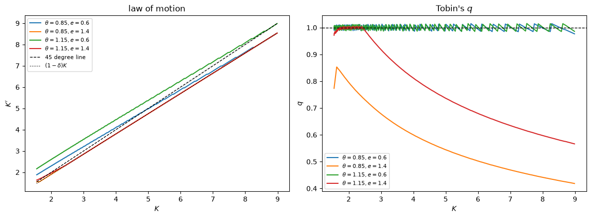
Fig. 115.1 Law of motion and Tobin’s q#
The law of motion runs along the lower dotted line \((1-\delta)K\) whenever the irreversibility constraint binds.
Exactly on that region, \(q\) falls below one.
115.6.2. The invariant distribution#
As in Investment Under Uncertainty, we check that the long-run distribution does not depend on where the economy starts.
def simulate(m, idx, K0, T=50_000, seed=0, burn=500):
    "Simulate the equilibrium Markov process."
    rng = np.random.default_rng(seed)
    j_idx = rng.integers(0, m.nθ, T)
    l_idx = rng.integers(0, m.ne, T)
    k = np.abs(m.K - K0).argmin()
    path = np.empty(T, int)
    for t in range(T):
        path[t] = k
        k = idx[k, j_idx[t], l_idx[t]]
    return path[burn:], j_idx[burn:], l_idx[burn:]

p_lo, j_lo, l_lo = simulate(m, idx, K0=2.0, seed=7)
p_hi, j_hi, l_hi = simulate(m, idx, K0=15.0, seed=7)

print(f"mean capital starting from K0 = 2:  {m.K[p_lo].mean():.4f}")
print(f"mean capital starting from K0 = 15: {m.K[p_hi].mean():.4f}")
print(f"capital visited: [{m.K[p_lo].min():.2f}, {m.K[p_lo].max():.2f}]")
mean capital starting from K0 = 2:  4.5395
mean capital starting from K0 = 15: 4.5395
capital visited: [2.06, 7.24]
fig, axes = plt.subplots(1, 2, figsize=(12, 4.5))

axes[0].hist(m.K[p_lo], bins=60, density=True, alpha=0.5, label='from $K_0 = 2$')
axes[0].hist(m.K[p_hi], bins=60, density=True, alpha=0.5, label='from $K_0 = 15$')
axes[0].set_xlabel('$K$'); axes[0].set_ylabel('density')
axes[0].set_title('invariant distribution of capital')
axes[0].legend()

q_sim, I_sim = q[p_lo, j_lo, l_lo], I[p_lo, j_lo, l_lo]
axes[1].scatter(q_sim, I_sim, s=4, alpha=0.2)
axes[1].set_xlabel('$q$'); axes[1].set_ylabel('$I$')
axes[1].set_title("investment and Tobin's $q$")

plt.tight_layout()
plt.show()
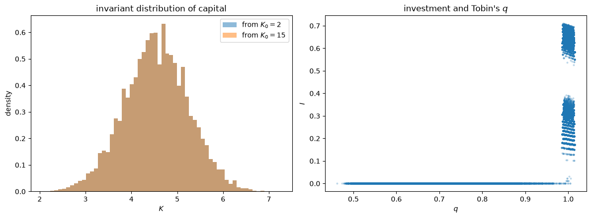
Fig. 115.2 Invariant distribution and investment against q#
The two histograms coincide, as Theorem 115.1 leads us to expect.
The scatter plot on the right reproduces the central picture of Sargent [1980].
Investment is positive only when \(q\) equals one; when \(q\) is below one, investment is exactly zero.
print(f"q when I > 0: [{q_sim[I_sim > 1e-12].min():.4f}, {q_sim[I_sim > 1e-12].max():.4f}]")
print(f"q when I = 0: [{q_sim[I_sim <= 1e-12].min():.4f}, {q_sim[I_sim <= 1e-12].max():.4f}]")
q when I > 0: [0.9851, 1.0148]
q when I = 0: [0.4619, 1.0040]
The small departures from exactly one reflect the discreteness of the capital grid.
Sargent’s point is now visible.
There is a positive relationship between investment and \(q\) in these data, and an econometrician could certainly run that regression.
But the relationship is not an investment demand schedule.
It is a mongrel relation that mixes together preferences, technology and the distribution of the shocks, and it will shift whenever any of them changes.
Exercise 115.3 asks you to demonstrate this.
115.7. Exercises#
Exercise 115.1
Brock and Mirman [1972] is famous partly for a special case that can be solved by hand.
Let \(u(c) = \ln c\), let \(f(k, r) = r k^\alpha\) with \(0 < \alpha < 1\), and let capital depreciate fully each period, so that \(k_{t+1} = f(k_t, r_t) - c_t\).
Verify that the optimal policy is \(k_{t+1} = \alpha\beta\, r_t k_t^\alpha\).
Show that \(\ln k_t\) follows an AR(1) process, and derive the mean and variance of its invariant distribution when \(\ln r_t \sim N(\mu, \sigma^2)\).
Simulate the model and check both the invariant distribution and the mean-ergodic property (115.5).
Solution
Guess that a constant fraction of resources is saved, \(k_{t+1} = s\, r_t k_t^\alpha\).
The Euler equation for this problem is
With \(c_t = (1-s) r_t k_t^\alpha\) and \(k_{t+1} = s r_t k_t^\alpha\), the right side becomes
while the left side is \(1/[(1-s) r_t k_t^\alpha]\).
Equating the two gives \(s = \alpha\beta\).
Taking logs of the policy,
an AR(1) with coefficient \(\alpha\).
With \(\ln r_t \sim N(\mu, \sigma^2)\), the invariant distribution of \(\ln k\) is normal with
α, β_d, μ, σ = 0.4, 0.95, 0.0, 0.1
T = 200_000
rng = np.random.default_rng(0)
ln_r = μ + σ * rng.normal(size=T)

k = np.empty(T + 1)
k[0] = 1.0
for t in range(T):
    k[t+1] = α * β_d * np.exp(ln_r[t]) * k[t]**α

ln_k = np.log(k[1000:])
print(f"mean of ln k: simulated {ln_k.mean():.4f}, "
      f"theory {(np.log(α*β_d) + μ)/(1-α):.4f}")
print(f"var  of ln k: simulated {ln_k.var():.4f}, "
      f"theory {σ**2/(1-α**2):.4f}")
mean of ln k: simulated -1.6126, theory -1.6126
var  of ln k: simulated 0.0119, theory 0.0119
The time averages match the population moments of the invariant distribution, which is the mean-ergodic property (115.5) in action.
Exercise 115.2
This exercise examines the difference between the two candidate formulas for \(v_K\) discussed above.
For the baseline model, compute at every state
the envelope formula (115.11)
the formula \(u_c(c,e)[f'(K)\theta + (1-\delta)]\)
a finite-difference derivative of the value function
Then
Confirm that all three agree where investment is positive.
Confirm that the second disagrees with the other two where investment is zero, and report by how much.
Explain, using (115.8), why the second formula is an upper bound for \(v_K\).
What would go wrong with the computed \(q\) if you used the second formula everywhere?
Solution
The second formula is what you get by substituting the first-order condition (115.8) into the envelope condition as though \(\lambda = 0\).
Since \(\lambda \geq 0\), dropping it can only raise the expression, so
with equality exactly when \(\lambda = 0\), that is, when investment is positive.
gap = np.abs(naive - vK_fd)/np.abs(vK_fd)
env = np.abs(vK - vK_fd)/np.abs(vK_fd)

for name, sel in (("investment positive", ~corner), ("investment zero", corner)):
    s = mid & sel
    print(f"{name:20}: envelope {np.median(env[s]):.4f}   "
          f"naive {np.median(gap[s]):.4f}   max naive {gap[s].max():.4f}")

q_naive = m.β * np.tensordot(naive, m.W, axes=([1, 2], [0, 1]))[idx] / u_c
print(f"\nusing the naive formula, max q = {q_naive.max():.3f} "
      f"(theory says q ≤ 1)")
print(f"fraction of states with q > 1: {(q_naive > 1 + 1e-8).mean():.3f}")
investment positive : envelope 0.0005   naive 0.0066   max naive 0.0134
investment zero     : envelope 0.0001   naive 0.3856   max naive 1.0175

using the naive formula, max q = 1.863 (theory says q ≤ 1)
fraction of states with q > 1: 0.578
Using the second formula everywhere produces values of \(q\) that exceed one, which the theory rules out.
The reason is economic, not numerical: at a corner the market does not price installed capital at the cost of new capital, precisely because the household would like to sell capital and cannot.
Exercise 115.3
Show that the regression of investment on \(q\) is not structural.
Solve and simulate the model for several economies that differ in
the amount of preference risk (the spread of \(e\))
the amount of technology risk (the spread of \(\theta\))
the depreciation rate \(\delta\)
For each economy, report the slope and \(R^2\) of a regression of \(I\) on \(q\), together with the frequency with which investment is zero.
Comment on what this implies for an econometrician who estimates an “investment demand schedule” relating investment to \(q\).
Solution
Here is one solution.
def q_regression(**kwargs):
    "Solve an economy, simulate it, and regress I on q."
    mm = create_model(**kwargs)
    vv, ii, _, II, CC = solve_model(mm)
    vvK = marginal_value(mm, ii, CC)
    uu_c = mm.e[None, None, :]/CC
    qq = mm.β * np.tensordot(vvK, mm.W, axes=([1, 2], [0, 1]))[ii] / uu_c
    p, j, l = simulate(mm, ii, K0=3.5)
    q_s, I_s = qq[p, j, l], II[p, j, l]
    slope = np.polyfit(q_s, I_s, 1)[0]
    corr = np.corrcoef(I_s, q_s)[0, 1]
    return slope, corr**2, (I_s <= 1e-12).mean()

cases = [("baseline",              {}),
         ("less preference risk",  dict(e_vals=(0.8, 1.2))),
         ("more preference risk",  dict(e_vals=(0.4, 1.6))),
         ("less technology risk",  dict(θ_vals=(0.95, 1.05))),
         ("more technology risk",  dict(θ_vals=(0.7, 1.3))),
         ("faster depreciation",   dict(δ=0.10))]

print(f"{'economy':24}{'slope':>9}{'R^2':>8}{'zero I':>9}")
for name, kw in cases:
    slope, r2, zero = q_regression(**kw)
    print(f"{name:24}{slope:9.3f}{r2:8.3f}{zero:9.3f}")
economy                     slope     R^2   zero I
baseline                    1.127   0.594    0.500
less preference risk        1.094   0.283    0.279
more preference risk        1.131   0.780    0.501
less technology risk        1.308   0.904    0.501
more technology risk        0.780   0.234    0.529
faster depreciation         1.271   0.436    0.456
The slope and the fit both move around substantially across economies that share the same preferences and technology parameters but differ in the distribution of shocks or in the depreciation rate.
Nothing in the regression is invariant, so it cannot be used to predict what investment would do under a policy that changed any of these features.
This is the message of Sargent [1980], and it is a concrete instance of the Lucas critique: the very friction that makes \(q\) interesting – the occasionally binding irreversibility constraint – also makes the relationship between \(I\) and \(q\) a reduced-form artifact rather than a decision rule.